Lab11 Localization(sim)

Grid Localization

The robot state is 3 dimensional and is given by [x, y, theta]. In this lab, the robot’s world is a continuous space that spans from[1]:

We discretize the continuous state space into a finite 3D grid space for the grid localization. Each grid cells are identical in size. In this lab, we chose the resolution of the grid to be 0.3048 m, 0.3048 meters, and 20 degrees along the x, y, and theta axes, respectively. Accordingly, the totala number of cells are 12*9*18.

The belief of the robot is therefore represented by the set of probabilities of each grid cell, and these probabilities should sum to 1.

Motion Model

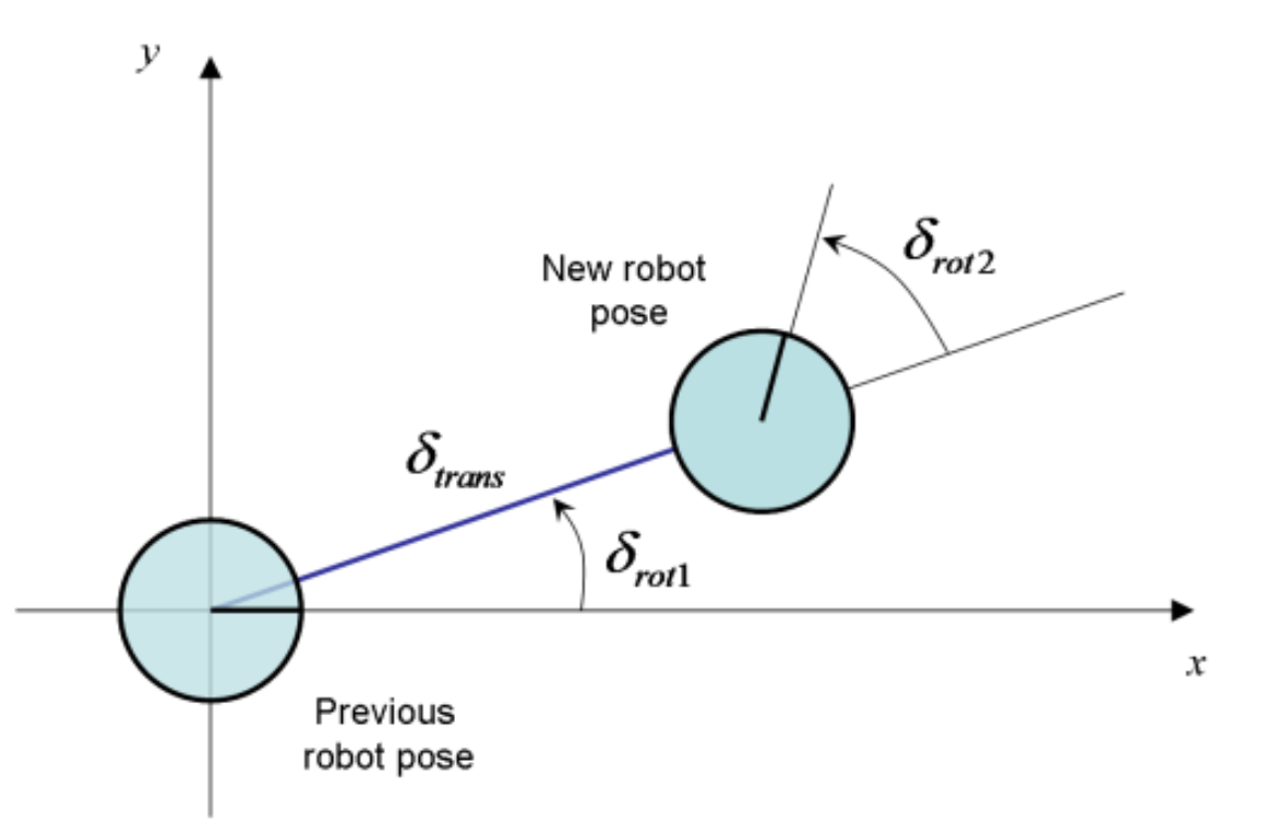
The odometry data before and after the movement is recorded at every timestamp. This relative odometry information can be described by the motion parameters: rotation1, translation, and rotation2.

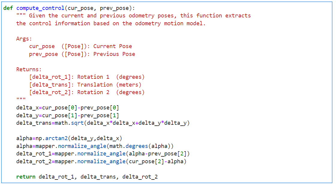
To go from one state to another, the robot will firstly turn a certain angle (rotation1), secondly go forward (translation), and do the final rotation (rotation2). I wrote the function compute_control to extract the control information from the odometry.

Given that the theta is in the range of [-180, +180) degrees, I used arctan2 and normalized the related output.

In this lab, we assume the process noise follows a Gaussian distribution. Given the rotation1, translation and rotation2 are independent, the p(x'|x, u) is:

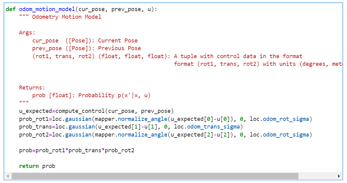
And I wrote a function odom_motion_model which returns the probability p(x'|x, u).

Sensor Model

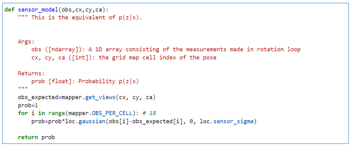
After reaching a new pose, the robot will rotate counterclockwise and get 18 measurements at the equidistant angular position. Compared with the expected measurements, we are able to correct the pose. Assuming individual measurements are independent and the noise is in gaussian distribution, the likelihood of P(z|x) is equal to:

The related code is shown below.

Bayes Filter

Bayes Filter is one of the fundamental approaches to estimating the distribution in a process with incoming measurements. There are two major steps:

Step1 Prediction: For all previous states, calculate the probability of becoming the current state given the input control, and add them up, noted as bel_bar.
Step2 Update Update the likelihood based on the measurements.

Prediction Step

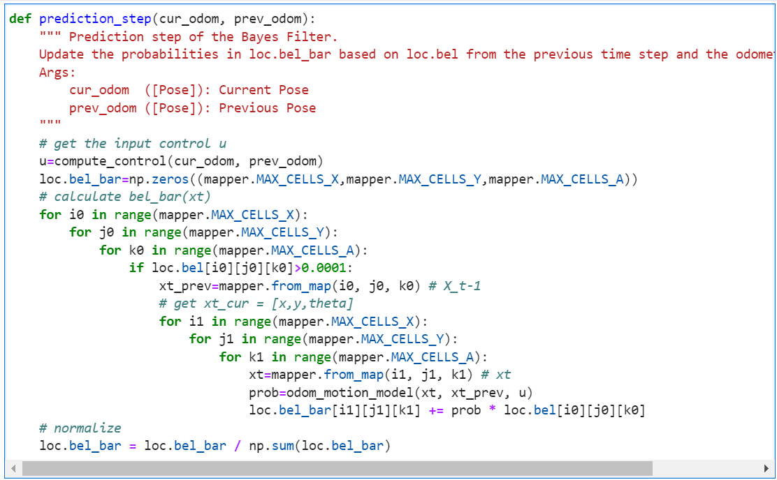
We need six 'for' loops to do the prediction step for all states: three for the current state, and another three for the previous state. Given that the grid has 12×9×18 possible states, the total loop number is 3,779,136, which will take a lot of time. To make the prediction more efficient, I set a threshold (0.0001) for the bel(x_prev). If the bel(x_prev) is less than the threshold, I will regard the robot can't be in this grid and skip it. That is to say, the inner three 'for' loops for getting the current states will not execute. Here is the related code.

Update Step

After the prediction, the Bayes Filter will update the probabilities based on the bel_bar and the sensor model. That is, for every state, the new likelihood is the bel_bar(xt) * p(z|x) and then normalize it. Here is the related code.

Demo

In the following video, odometry(red line), ground truth(green line), belief(blue line), and bel_bar(gray grids) are plotted together. The lighter the gird, the larger the bel_bar is. We can tell that the Bayes Filter can be done in just two minutes and the results are close to the ground truth. Additionally, the bel_bar after the predictions are not so good but the update step is able to decrease the errors.

References

[1].Fast Robots Lab11 Guidance

Posted by Lanyue Fang on Apr 25, 2022